Conic Lagrangians in frequency coordinates

This companion supplies the geometric coordinate theorem needed by the frequency-graph criterion. It proves a statement about a change of base coordinates and its cotangent lift. Transporting an operator class under that change, or cutting a distribution off microlocally, requires additional analytic proofs.

The freely readable source is Lars Hörmander's Fourier integral operators. I, Section 3.1, especially Theorems 3.1.3 and 3.1.4, printed pages 134–137. The original paper is freely available. The arguments below include the finite-dimensional and chart details used here; the reference does not replace any of those proofs.

C0. Exact inputs and conventions

We work in dimension $n\ge1$. A smooth embedded $n$-dimensional submanifold means a set locally given by an injective smooth parametrization with a smooth inverse onto its image, whose derivative has rank $n$. Its tangent space is the image of that derivative. A conic set is invariant under every positive dilation of the frequency variable, leaving the base variable fixed.

The earlier programme proofs are:

Their exact source bytes, actual proof locators and transitive dependencies are recorded in the companion proof bindings. All uses of inverse or implicit maps below are finite-dimensional applications of P3. No general normal-form theorem or theorem about closed one-forms is imported.

The finite rank facts used below. If $A:V\to W$ is linear, choose a basis of $\ker A$ and extend it to a basis of $V$. The images of the added vectors span $A(V)$. They are independent: a linear combination with zero image belongs to $\ker A$, so independence of the full basis makes its added coefficients zero. It follows that $\dim V=\dim\ker A+\dim A(V)$. In particular a linear injection between spaces of the same finite dimension is an isomorphism. If the rows of a real $N$-by-$d$ matrix are independent, its image is all of $\mathbb R^N$. Otherwise an orthogonal complement of its proper image contains a nonzero vector, giving a nonzero linear combination of the rows equal to zero. The columns therefore span, and a basis chosen from them gives an invertible $N$-column minor. If a $d$-by-$n$ matrix is injective, its rows span $\mathbb R^n$: a nonzero vector perpendicular to all the rows would be in its kernel. Choosing a basis of rows gives an invertible $n$-row minor. These arguments use the basis-extension and orthonormal-complement proofs cited above, and supply every rank, nullity and minor-selection fact used in C1, C3 and C5.

For tangent vectors $(v,w)$ and $(v',w')$, use

Thus $\omega=\sum_jd\xi_j\wedge dx_j$. An $n$-plane is Lagrangian when $\omega$ vanishes on it. A smooth $n$-submanifold is Lagrangian when every tangent plane has this property.

If $x=f(y)$ is a base diffeomorphism, write $J=df_y$. The frequency coordinates obey

This identity follows by pairing with every vector $dy$: $\eta\cdot dy=\xi\cdot J\,dy=\xi\cdot dx$. It proves invariance of $\alpha$. It also proves invariance of $\omega$ directly: differentiating (C2), the extra term in $\sum_jd\eta_j\wedge dy_j$ has coefficients $\sum_k\xi_k\partial_{y_\ell}\partial_{y_j}f_k$. They are symmetric in $j,\ell$, so their contributions to the alternating form cancel in pairs. The remaining term is $\sum_kd\xi_k\wedge dx_k$. The smooth inverse in (C2) is supplied by P2. This verifies the cotangent lift without an exterior-calculus identity left as a prerequisite.

C1. A horizontal graph transverse to a Lagrangian plane

Lemma. Let $L$ be a Lagrangian $n$-plane in $\mathbb R_y^n\oplus\mathbb R_\eta^n$. There is a real $t$ such that

This graph is also transverse to the vertical plane $q=0$.

Proof. Let $E$ be the image of the base projection $L\to\mathbb R^n$, of dimension $k$, and let $V=\{p:(0,p)\in L\}$. For $p\in V$ and $q\in E$, choose $(q,r)\in L$. Isotropy gives $p\cdot q=0$; hence $V\subset E^\perp$. Rank and nullity give $\dim V=n-k=\dim E^\perp$, so these two spaces are equal. The orthogonal complement has that dimension because an orthonormal basis of $E$ extends to one of $\mathbb R^n$, by the finite Gram–Schmidt proof P9.4.

For $q\in E$, choose $(q,p)\in L$ and define $Bq$ to be the orthogonal projection of $p$ on $E$. Any other choice differs by an element of $V=E^\perp$, so $Bq$ is well-defined. Addition and scalar multiplication in $L$ show that $B$ is linear. Isotropy applied to two such lifts gives $(Bq)\cdot q'=q\cdot(Bq')$; thus $B$ is symmetric. In fact

Both inclusions follow from the definition and from $\{0\}\oplus E^\perp\subset L$.

If $k=0$, the plane $L$ is vertical and any $t$ works. Otherwise, in an orthonormal basis of $E$, let $C=k\max_{i,j}|B_{ij}|$. Each component of $Bq$ is at most $\max|B_{ij}|\sum_j|q_j|$; Cauchy–Schwarz therefore gives $|Bq|\le C|q|$. Choose $t=C+1$. If $(q,tq)\in L$, then $q\in E$ and projection of (C4) onto $E$ gives $tq=Bq$. The bound forces $q=0$. This proves (C3). The graph itself is Lagrangian because $(tq)\cdot q'-(tq')\cdot q=0$, and it has dimension $n$. Its intersection with the vertical plane is zero by its definition. $\square$

This is the particular common-transversal statement the coordinate construction needs. It uses only real linear algebra and avoids importing a parametrization of all Lagrangian planes.

C2. The radial vector kills the canonical one-form

At $(y,\eta)$ on a conic Lagrangian $\Lambda$, the curve $s\mapsto(y,s\eta)$ lies in $\Lambda$. Its derivative at $s=1$ is $R=(0,\eta)$, so $R\in T\Lambda$. For every tangent $(v,w)\in T\Lambda$, (C1) gives

Consequently $\alpha$ vanishes on $\Lambda$. This proof uses conicity as well as the Lagrangian hypothesis.

C3. Construct the base coordinates and the conic chart

Theorem. Given a conic embedded Lagrangian $\Lambda\subset T^*X\setminus0$ and a point $\rho\in\Lambda$, there are base coordinates $x$ near $\pi(\rho)$, an open cone $\Omega\subset\mathbb R^n\setminus0$, and a smooth degree-zero map $g:\Omega\to\mathbb R^n$ such that the conic germ of $\Lambda$ at the positive ray of $\rho$ is

In particular the change comes from a base diffeomorphism.

Proof. Start with coordinates $y$ centered at $\pi(\rho)$ in which the covector at $\rho$ is $dy_1$. To obtain them, extend that nonzero covector to a basis of the dual vector space and use those linear functions as coordinates. Thus $\rho=(0,e_1)$. Apply C1 to $L=T_\rho\Lambda$, and fix the resulting $t$. Define

Its derivative at zero is the identity, so P3 makes this a smooth base diffeomorphism on a sufficiently small neighborhood.

The section $\eta=d_yx_1=e_1+ty$ has tangent plane $M_t$ at $\rho$. In the new cotangent coordinates it is the section $\xi=e_1$, by (C2). Equivalently, differentiating $\eta=(df_y)^T\xi$ at $(y,\xi)=(0,e_1)$ gives

Thus the kernel of $d\xi$ is precisely $M_t$. Since $M_t\cap T_\rho\Lambda=0$, the restriction $d\xi:T_\rho\Lambda\to\mathbb R^n$ is injective and hence an isomorphism. C0 shows that $\Lambda$ is still Lagrangian in the new coordinates.

Here is the passage from an ordinary inverse chart to a conic one. Work where $\xi_1>0$, and use ambient coordinates

This is a smooth coordinate map with the explicit inverse $(x,\nu,s)\mapsto(x,s(1,\nu))$. Conicity says that membership in $\Lambda$ is unchanged by varying $s$ with $(x,\nu)$ fixed. The section $\Lambda_1=\Lambda\cap\{\xi_1=1\}$ is smooth of dimension $n-1$: $d\xi_1(R)=1$ on that section, and the implicit map theorem in a parametrization of $\Lambda$ solves for this one coordinate. On its tangent space at $\rho$, $d\nu=d\xi'$. If $d\nu$ vanishes, so does all of $d\xi$, and the tangent vector is zero. Dimension now makes this map an isomorphism. P3 therefore gives a unique local chart

after shrinking an open neighborhood $V$ of $0$. When $n=1$, this section is a single point and (C10) is the corresponding zero-dimensional chart.

Saturate this chart by positive dilation. In the product coordinates (C9), it is an open part of $\Lambda$, containing the entire positive ray of $\rho$. Its frequency image is the open cone $\Omega=\{s(1,\nu):s>0,\ \nu\in V\}$. Set $g(s(1,\nu))=g_1(\nu)$. This map is smooth and degree zero, and gives (C6). All charts can be restricted in the base variable, so the chosen base coordinate neighborhood is respected. $\square$

C4. The homogeneous generating function and its extension

Define

C2, applied to the chart (C6), says $\sum_j\xi_j\,dg_j=0$. The product rule then gives

Thus $H'=g$. Since $g(s\xi)=g(\xi)$, the function $H$ is homogeneous of degree one. Conversely, if a degree-one smooth function $K$ has $K'=g$, differentiating $K(s\xi)=sK(\xi)$ at $s=1$ gives $K(\xi)=\xi\cdot K'(\xi)=\xi\cdot g(\xi)=H(\xi)$. This proves uniqueness, including the additive constant. Differentiating $H'(s\xi)=H'(\xi)$ also gives

For the analytic receiver, a globally defined homogeneous extension may be chosen after shrinking the angular cone. Take an open $V_0$ with compact closure inside $V$. U001 Appendix A.4 supplies a smooth $\beta$, supported in $V$, equal to one near $\overline V_0$, with compact support in that ratio chart. Put $h(\nu)=H(1,\nu)$ and define

The product $\beta h$ extends smoothly by zero outside $V$, by the strictly interior support. Its support has $|\xi'|/\xi_1\le M$ for some finite $M$. At any nonzero point with $\xi_1=0$, a sufficiently small neighborhood has $|\xi'|>M\xi_1$ whenever $\xi_1>0$; hence (C14) is zero there. This proves smoothness across that boundary. It is visibly smooth elsewhere and homogeneous of degree one. All derivatives of $H$ and $\widetilde H$ agree on a neighborhood of the smaller cone. For $n=1$, take $\beta=1$ on the one-point ratio space; the two half-lines are separate components of $\mathbb R\setminus0$, so the same conclusion holds.

The graph phase

has critical equations $\phi_\theta'=x-H'(\theta)=0$. Their derivatives in $x$ form the identity matrix, so they are independent. Moreover $\phi_x'=\theta\ne0$. Its critical map is exactly $(x,\theta)\mapsto(H'(\theta),\theta)$. This proves directly that it is a nondegenerate phase for the germ (C6). The extension in (C14) changes none of these statements in the smaller cone. It makes no claim about the Lagrangian outside that cone.

C5. The geometry supplied by any nondegenerate phase

Let $\phi(x,\theta)$ be real and smooth on an open cone in $\mathbb R^n\times(\mathbb R^N\setminus0)$, homogeneous of degree one in $\theta$. Suppose its full differential is nonzero, and the $N$ differentials $d(\partial_{\theta_j}\phi)$ are independent on $C_\phi=\{\phi_\theta'=0\}$. Then the critical map

is locally an embedding onto a conic Lagrangian.

Proof. Choose an invertible $N$-column minor of the derivative of $\phi_\theta'$. The implicit map theorem solves for those $N$ variables, leaving a smooth $n$-dimensional critical chart. Its tangent equation is

If $d\kappa(v,w)=0$, then $v=0$ and $\phi_{x\theta}''w=0$; (C17) adds $\phi_{\theta\theta}''w=0$. Mixed-partial symmetry says this is the transpose of the full $N$-row derivative of $\phi_\theta'$ applied to $w$. Independence of those rows forces $w=0$. Thus $d\kappa$ is injective. In critical-chart coordinates choose $n$ output components whose derivative minor is invertible. Applying P3 to those components makes the remaining output components smooth functions of them. This gives the asserted local embedding, without invoking a separate immersion theorem.

At a critical point, nonvanishing of the full differential implies $\phi_x'\ne0$, so the image avoids the zero section. The equation $\phi_\theta'(x,s\theta)=\phi_\theta'(x,\theta)$ and $\phi_x'(x,s\theta)=s\phi_x'(x,\theta)$ prove conicity of its saturated local germ. Euler's identity gives $\phi=\theta\cdot\phi_\theta'=0$ on $C_\phi$. Consequently the differential of its restriction is zero: $\phi_x'\cdot dx=0$ on every critical tangent. To see isotropy explicitly, write a critical chart as $t\mapsto(x(t),\theta(t))$ and $\zeta(t)=\phi_x'(x(t),\theta(t))$. Then $\sum_j\zeta_j\partial_{t_a}x_j=0$. Differentiate in $t_b$, subtract the equation with $a,b$ reversed, and cancel the mixed derivatives of $x_j$. The result is the vanishing of (C1) on those two image tangents. The image has dimension $n$, so it is Lagrangian. $\square$

There is also an exact rank identity at each critical point:

Indeed $d\kappa$ is a tangent isomorphism onto the image. The kernel of $d\pi$ therefore corresponds to the vectors $(0,w)$ satisfying (C17), namely $\ker\phi_{\theta\theta}''$. Rank and nullity on these two finite-dimensional spaces prove (C18). Euler's identity differentiated in $\theta$ gives $\phi_{\theta\theta}''\theta=0$. Since $\theta\ne0$, the common nullity is at least one, as conicity also requires.

C6. An exact model and two exercises

Take the positive conormal of the line $y_1=0$ in $\mathbb R^2$:

At $s=0,\lambda=1$, choose $t=1$ in (C7). Formula (C2), with $df_y=\begin{pmatrix}1+y_1&y_2\\0&1\end{pmatrix}$, gives

The old frequency projection loses $s$; the new one recovers $\lambda=\xi_1$ and $s=-\xi_2/\xi_1$. The generating function is

Its gradient is $(\xi_2^2/(2\xi_1^2),-\xi_2/\xi_1)$, exactly (C20). These are a line and a parabola in the respective base coordinates; the full Lagrangians also contain the indicated positive covector rays.

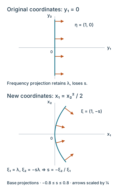
Figure C1. Base projections of (C19) and (C20) for $-0.8\le s\le0.8$. The arrows display the Euclidean representatives of the exact covectors with $\lambda=1$, multiplied by the same positive plotting factor $0.25$. They are normal to their respective curves, not trajectory arrows. Equations (C19)–(C21) give all coordinates and prove the conversion. The human source for the general construction is the free paper cited above, Theorem 3.1.3.

Exercise C1: verify that this coordinate change is a base diffeomorphism. Give its inverse near zero and check both the Jacobian and the covector law.

Solution. We have $y_2=x_2$ and $(1+y_1)^2=1+2x_1-x_2^2$. Near zero the right side is positive, and the branch with $y_1=0$ at $x=0$ is $y_1=-1+\sqrt{1+2x_1-x_2^2}$. Its smoothness follows from the earlier smooth-root proof in F0-DIFF. Substitution proves both inverse identities. The determinant of $df_y$ is $1+y_1$, nonzero there. On $y_1=0,y_2=s$, $(df_y)^T(\lambda,-s\lambda)=(\lambda,0)$, exactly (C2). $\square$

Exercise C2: identify the radial degeneracy of the model phase. For $\phi=x\cdot\theta-H(\theta)$ with (C21), determine the rank of $\phi_{\theta\theta}''$ and of the base projection of its critical Lagrangian.

Solution. Direct differentiation gives

It has rank one since $\xi_1>0$, and its kernel is the radial line spanned by $\xi$. Therefore $\phi_{\theta\theta}''=-H''$ also has rank one. The base projection in (C20) has derivative $\partial_sx=(s,1)\ne0$ and $\partial_\lambda x=0$, so its rank is one. Both sides of (C18) equal $2-1=1$. $\square$

What this component supplies

C3–C4 supply the geometric frequency graph in a base coordinate chart. C5 supplies the local critical-map geometry and its rank identity. These facts are proved relative to the exact earlier programme inputs in C0. The general intrinsic lesson still needs the analytic coordinate and microlocal localization proofs, its prescribed nondegenerate and clean phase representation results, its refined order theorem, and its full examples and exercises. Global density and Maslov transitions remain a separate requirement.

This companion and its figure were written by GPT-6 Astra (OpenAI), Ultra, 4 October 2026. Original exposition: CC0. It uses mathematical results from the freely readable source identified above; no source prose or source figure is reproduced. Earlier linked components keep their separately recorded authorship and licences.